import numpy as np
from sys import path

import matplotlib.pyplot as plt
import matplotlib as mpl
mpl.rcParams['lines.markersize'] = 6
mpl.rcParams['scatter.marker'] = '.'

path.append('../../')
import derivative

def plot_example(diff_method, t, data_f, res_f, sigmas, y_label=None):
    '''Utility function for concise plotting of examples.'''
    fig, axes = plt.subplots(1, len(sigmas), figsize=[len(sigmas)*4, 3])

    # Compute the derivative
    res = diff_method.d(np.vstack([data_f(t, s) for s in sigmas]), t, axis=1)
    for i, s in enumerate(sigmas):
        axes[i].plot(t, res_f(t))
        axes[i].plot(t, res[i])
        axes[i].set_title(r"Noise: $\sigma$={}".format(s))
        axes[i].set_ylim([-1.25,1.3])
    if y_label:
        axes[0].set_ylabel(y_label, fontsize=12)

Usage

There are two ways to interact with the code.

t = np.linspace(0, 2, 50)
x = np.sin(2*np.pi*t)

The first way is to do a specific import of the desired Derivative object.

from derivative import FiniteDifference

fig,ax = plt.subplots(1, figsize=[5,3])
kind = FiniteDifference(k=1)
ax.plot(t, kind.d(x,t));

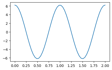
The second way is top use the functional interface and pass the kind of derivative as an argument.

# Use the functional interface and pass the kind as an argument
from derivative import dxdt

fig,ax = plt.subplots(1, figsize=[5,3])
ax.plot(t, dxdt(x, t, "finite_difference", k=1));

Examples

Smooth Derivative

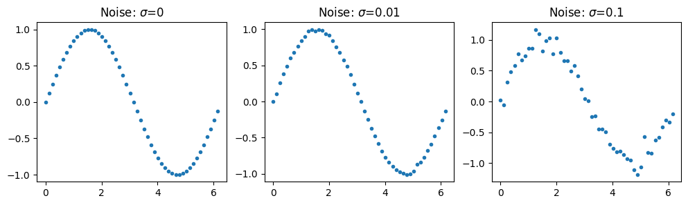
The first example is a sine function with Gaussian noise.

def noisy_sin(t, sigma):
    '''Sine with gaussian noise.'''
    np.random.seed(17)
    return np.sin(t) + np.random.normal(loc=0, scale=sigma, size=t.shape)

sigmas = [0, 0.01, 0.1]
fig, ax = plt.subplots(1, len(sigmas), figsize=[len(sigmas)*4, 3])

t = np.linspace(0, 2*np.pi, 50, endpoint=False)
for axs, s in zip(ax, sigmas):
    axs.scatter(t, noisy_sin(t, s))
    axs.set_title(r"Noise: $\sigma$={}".format(s))

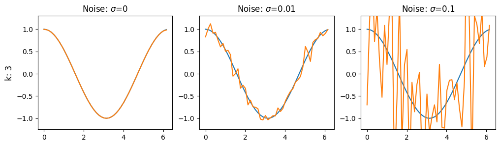
Finite differences

fd = derivative.FiniteDifference(3)
plot_example(fd, t, noisy_sin, np.cos, sigmas, 'k: 3')

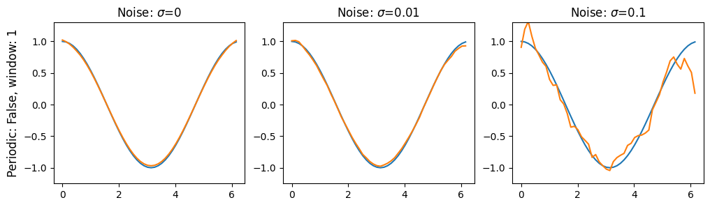
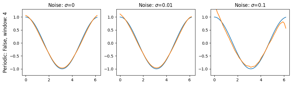
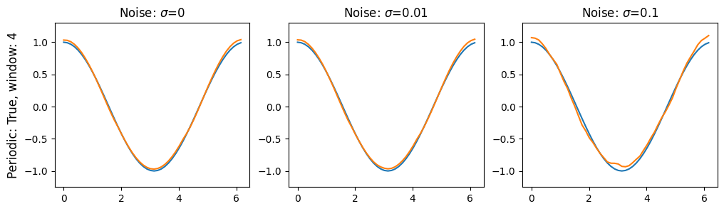
Savitzky-Golay filter

sg = derivative.SavitzkyGolay(left=.5, right=.5, order=2, periodic=False)
plot_example(sg, t, noisy_sin, np.cos, sigmas, 'Periodic: False, window: 1')

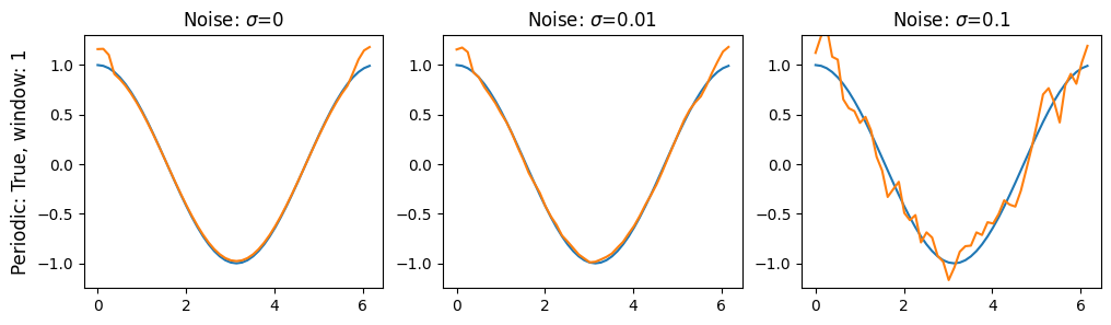
sg = derivative.SavitzkyGolay(left=.5, right=.5, order=2, periodic=True)
plot_example(sg, t, noisy_sin, np.cos, sigmas, 'Periodic: True, window: 1')

sg = derivative.SavitzkyGolay(left=2, right=2, order=3, periodic=False)
plot_example(sg, t, noisy_sin, np.cos, sigmas, 'Periodic: False, window: 4')

sg = derivative.SavitzkyGolay(left=2, right=2, order=3, periodic=True)
plot_example(sg, t, noisy_sin, np.cos, sigmas, 'Periodic: True, window: 4')

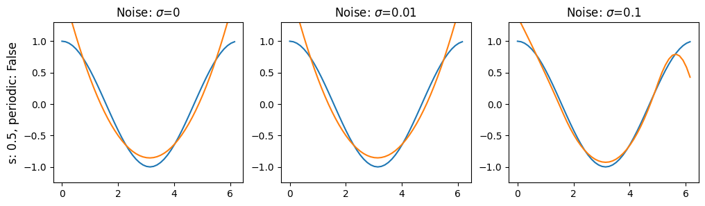
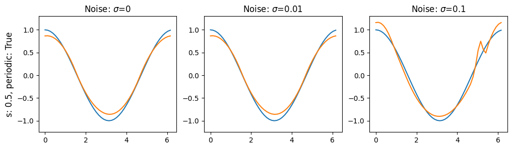
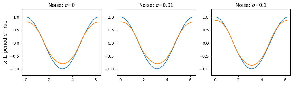
Splines

spl = derivative.Spline(.5)
plot_example(spl, t, noisy_sin, np.cos, sigmas, 's: 0.5, periodic: False')
spl = derivative.Spline(.5, periodic=True)
plot_example(spl, t, noisy_sin, np.cos, sigmas, 's: 0.5, periodic: True')
spl = derivative.Spline(1, periodic=True)
plot_example(spl, t, noisy_sin, np.cos, sigmas, 's: 1, periodic: True')

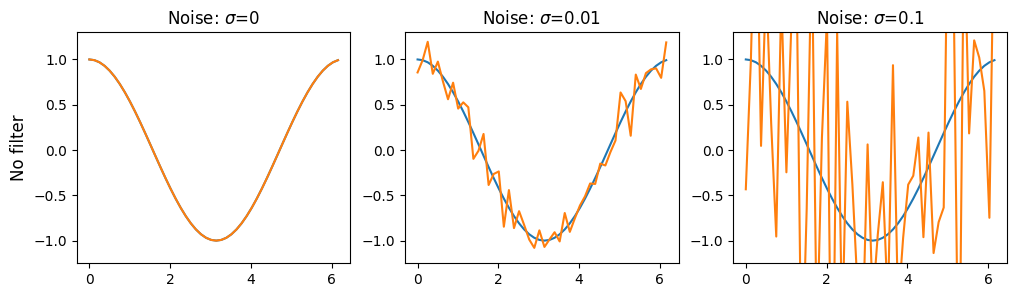
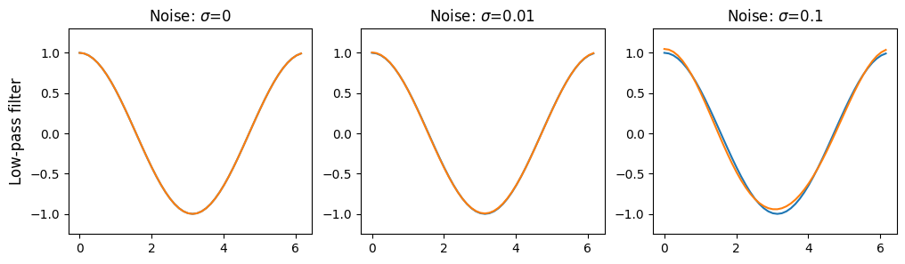
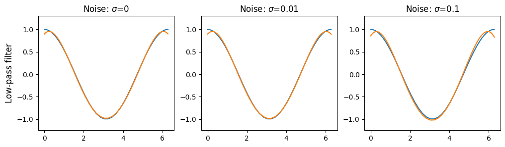
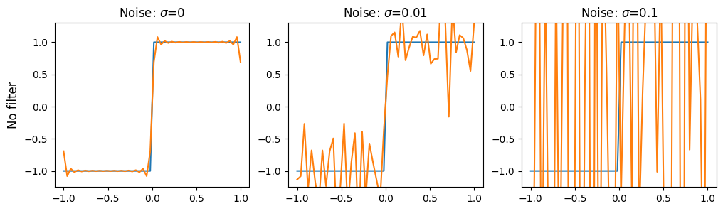
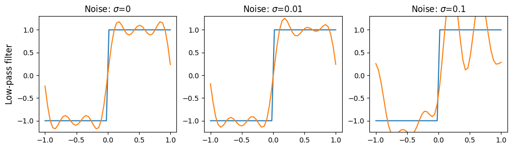
Spectral method - Fourier basis

Add your own filter!

no_filter =  derivative.Spectral()
yes_filter = derivative.Spectral(filter=np.vectorize(lambda k: 1 if abs(k) < 3 else 0))

plot_example(no_filter, t, noisy_sin, np.cos, sigmas, 'No filter')
plot_example(yes_filter, t, noisy_sin, np.cos, sigmas, 'Low-pass filter')

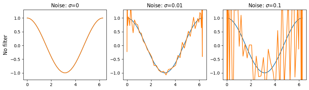
Spectral method - Chebyshev basis

Now let’s do with the Chebyshev basis, which requires cosine-spaced points on [a, b] rather than equispaced points on [a, b)

t_cos = np.cos(np.pi * np.arange(50) / 49) * np.pi + np.pi # choose a = 0, b = 2*pi
no_filter = derivative.Spectral(basis='chebyshev')
yes_filter = derivative.Spectral(basis='chebyshev', filter=np.vectorize(lambda k: 1 if abs(k) < 6 else 0))

plot_example(no_filter, t_cos, noisy_sin, np.cos, sigmas, 'No filter')
plot_example(yes_filter, t_cos, noisy_sin, np.cos, sigmas, 'Low-pass filter')

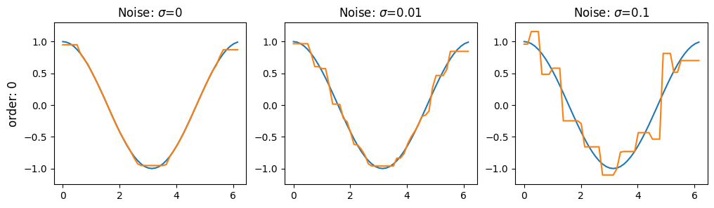
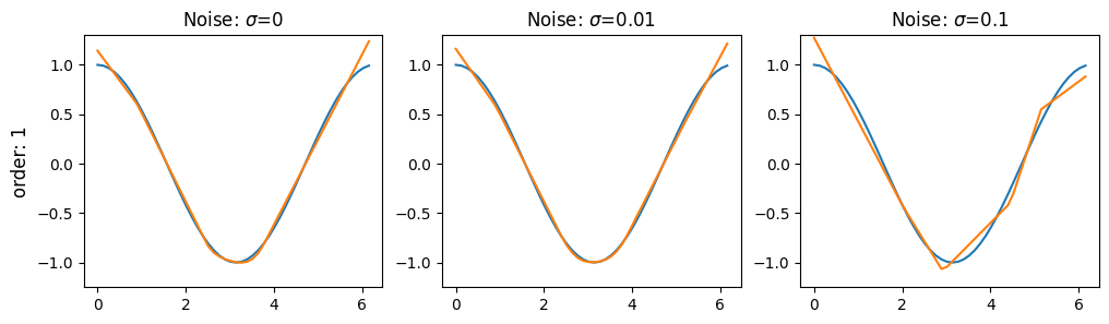
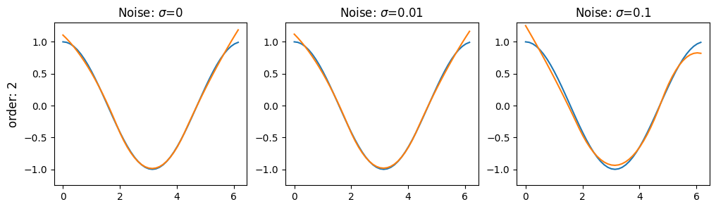
Trend-filtered

tvd =  derivative.TrendFiltered(alpha=1e-3, order=0, max_iter=int(1e6))
plot_example(tvd, t, noisy_sin, np.cos, sigmas, 'order: 0')

tvd =  derivative.TrendFiltered(alpha=1e-3, order=1, max_iter=int(1e6))
plot_example(tvd, t, noisy_sin, np.cos, sigmas, 'order: 1')

tvd =  derivative.TrendFiltered(alpha=1e-3, order=2, max_iter=int(1e6))
plot_example(tvd, t, noisy_sin, np.cos, sigmas, 'order: 2')

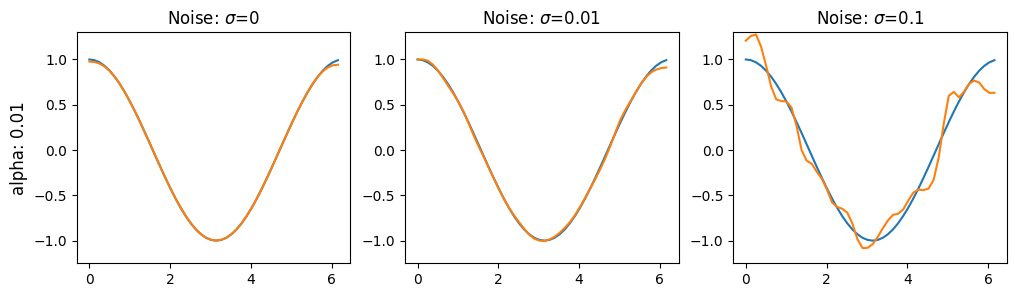
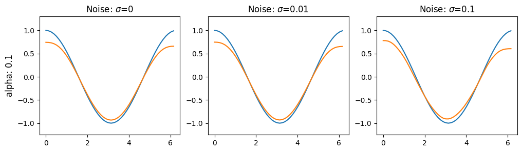
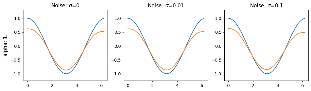
Kalman smoothing

kal =  derivative.Kalman(alpha=0.01)
plot_example(kal, t, noisy_sin, np.cos, sigmas, 'alpha: 0.01')

kal =  derivative.Kalman(alpha=0.5)
plot_example(kal, t, noisy_sin, np.cos, sigmas, 'alpha: 0.1')

kal =  derivative.Kalman(alpha=1)
plot_example(kal, t, noisy_sin, np.cos, sigmas, 'alpha: 1.')

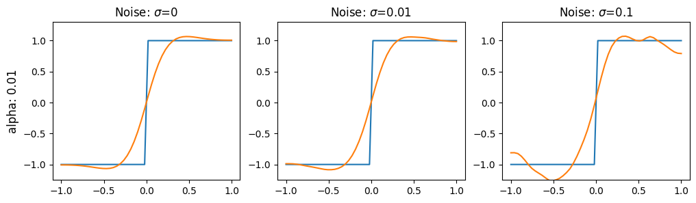
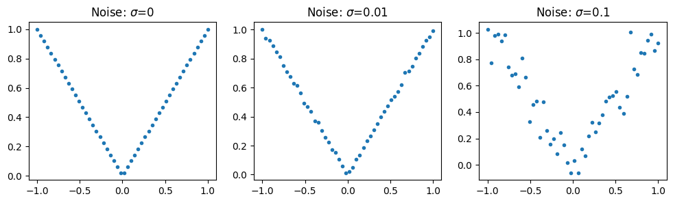
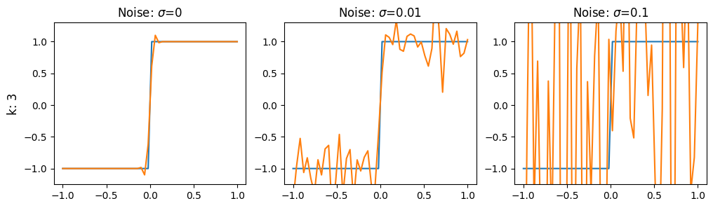
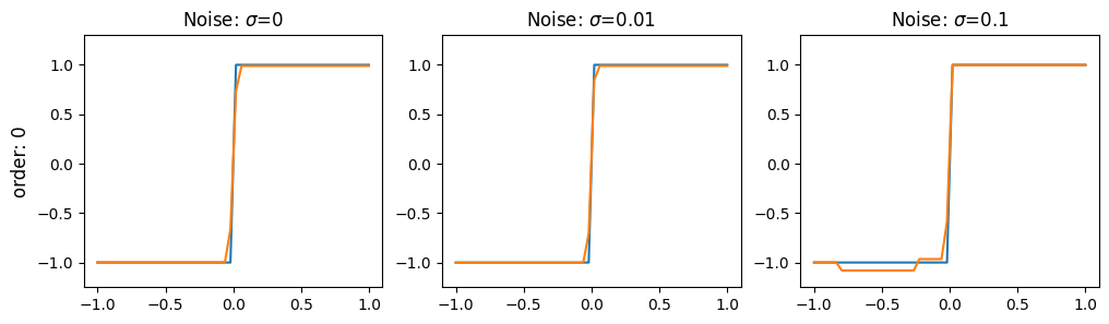
Jump Derivative

The second example is the absolute value function with Gaussian noise.

def noisy_abs(t, sigma):
    '''Abs with gaussian noise.'''
    np.random.seed(17)
    return np.abs(t) + np.random.normal(loc=0, scale=sigma, size=x.shape)

d_abs = lambda t: t/abs(t)

sigmas = [0, 0.01, 0.1]
fig, ax = plt.subplots(1, len(sigmas), figsize=[len(sigmas)*4, 3])

t = np.linspace(-1, 1, 50)
for axs, s in zip(ax, sigmas):
    axs.scatter(t, noisy_abs(t, s))
    axs.set_title(r"Noise: $\sigma$={}".format(s))

Finite differences

fd = derivative.FiniteDifference(k=3)
plot_example(fd, t, noisy_abs, d_abs, sigmas, 'k: 3')

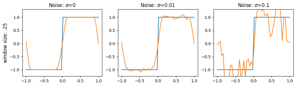
Savitzky-Galoy filter

sg = derivative.SavitzkyGolay(left=.125, right=.125, order=2, periodic=True, T=2)
plot_example(sg, t, noisy_abs, d_abs, sigmas, 'window size: .25')

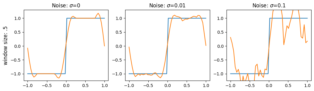
sg = derivative.SavitzkyGolay(left=.25, right=.25, order=3, periodic=True, T=2)
plot_example(sg, t, noisy_abs, d_abs, sigmas, 'window size: .5')

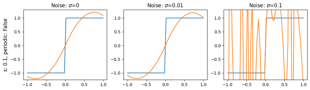
Splines

spl = derivative.Spline(.1, periodic=False)
plot_example(spl, t, noisy_abs, d_abs, sigmas, 's: 0.1, periodic: False')

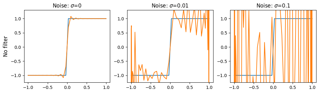
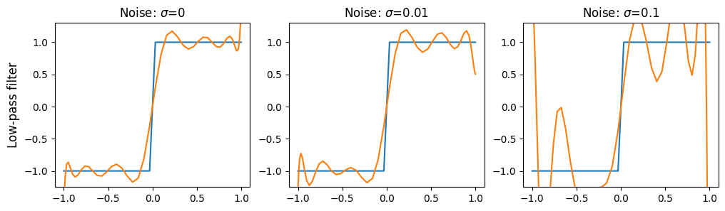
Spectral method - Fourier basis

no_filter =  derivative.Spectral()
yes_filter = derivative.Spectral(filter=np.vectorize(lambda k: 1 if abs(k) < 6 else 0))

plot_example(no_filter, t, noisy_abs, d_abs, sigmas, 'No filter')
plot_example(yes_filter, t, noisy_abs, d_abs, sigmas, 'Low-pass filter')

Spectral method - Chebyshev basis

t_cos = np.cos(np.pi * np.arange(50)/49)
no_filter = derivative.Spectral(basis='chebyshev')
yes_filter = derivative.Spectral(basis='chebyshev', filter=np.vectorize(lambda k: 1 if abs(k) < 15 else 0))

plot_example(no_filter, t_cos, noisy_abs, d_abs, sigmas, 'No filter')
plot_example(yes_filter, t_cos, noisy_abs, d_abs, sigmas, 'Low-pass filter')

Trend-filtered

tvd =  derivative.TrendFiltered(alpha=1e-3, order=0, max_iter=int(1e5))
plot_example(tvd, t, noisy_abs, d_abs, sigmas, 'order: 0')

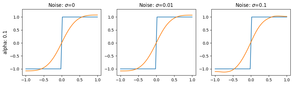
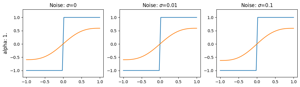
Kalman smoothing

kal =  derivative.Kalman(alpha=0.01)
plot_example(kal, t, noisy_abs, d_abs, sigmas, 'alpha: 0.01')

kal =  derivative.Kalman(alpha=0.1)
plot_example(kal, t, noisy_abs, d_abs, sigmas, 'alpha: 0.1')

kal =  derivative.Kalman(alpha=1.)
plot_example(kal, t, noisy_abs, d_abs, sigmas, 'alpha: 1.')